Stop Codon Frequency Analyser

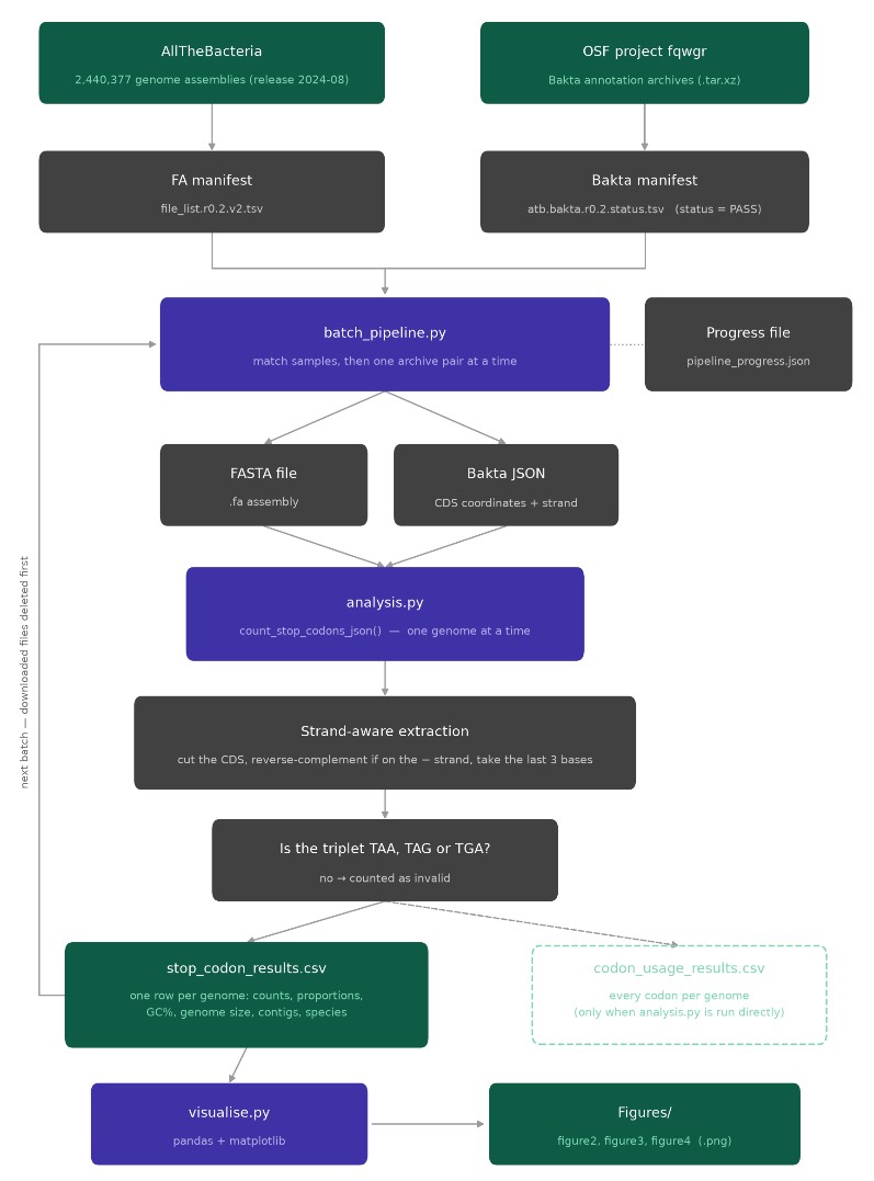
The system splits in two. An analysis module handles one genome at a time and can be pointed at a single pair of files; a batch pipeline handles fetching, matching and cleanup. Keeping them apart meant the extraction logic could be run and checked in isolation.

Each genome arrives as a FASTA assembly plus a Bakta JSON annotation giving CDS coordinates and strand. For every annotated coding sequence the module takes the terminal triplet: the last three bases on the positive strand, or the reverse complement of the first three on the negative, since Bakta records negative-strand features by their position on the forward sequence. Bakta's coordinates are one-based and inclusive, so each one is converted to Python's zero-based indexing.

The full archive set would have needed roughly 150 GB of disk, which was not available, so the pipeline pulls one archive pair at a time, processes it, and deletes it before moving on. Rows are appended to the CSV as they are produced rather than held in memory, so an interrupted run resumes without losing completed genomes. Bakta archive URLs are discovered at run time through the AllTheBacteria OSF API instead of being hardcoded.

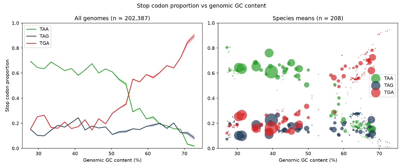
Across the 202,388 genomes TAA was the most common stop codon at 56.45% (302,692,618 counts), then TGA at 26.73% (143,325,034) and TAG at 16.81% (90,152,726). GC content ranged from 26.89% to 73.61% with a mean of 40.47%.

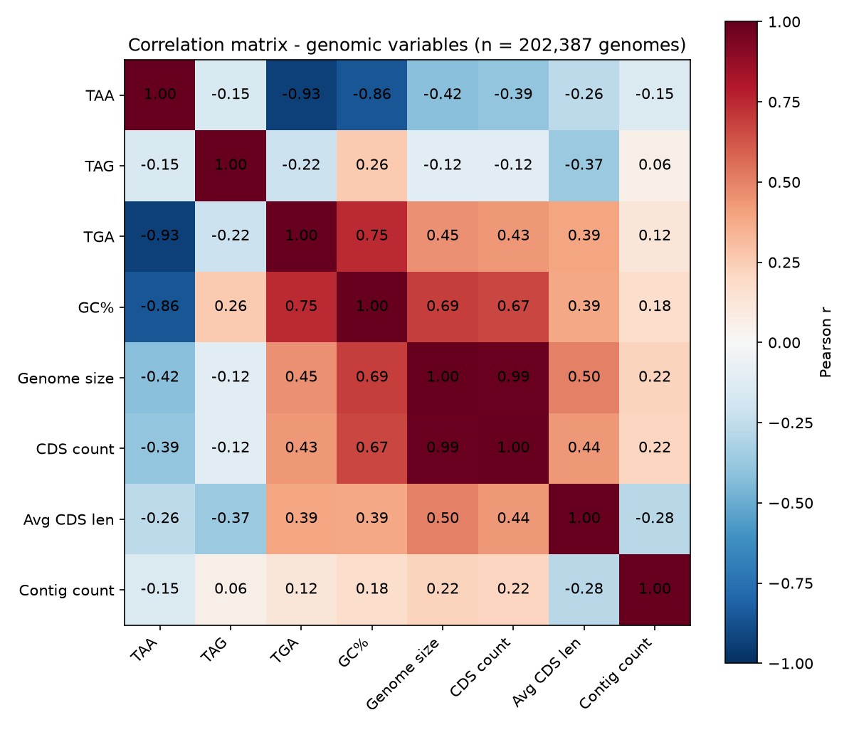
The correlation with base composition is strong and in the direction theory predicts: r = -0.855 between GC content and TAA usage, r = 0.749 for TGA. These are the two largest coefficients anywhere in the matrix. At species level the effect is starker still. Brachybacterium muris averages a TGA proportion of 0.910 at 70.0% GC, several Burkholderia species run 0.71 to 0.78 at 67-68% GC, and at the other end Brachyspira hyodysenteriae averages 0.805 TAA at just 27.1% GC.

TAG behaves differently. It stays roughly flat across the whole GC range, correlating only weakly with composition at r = 0.259, which suggests it is under less compositional pressure than the other two.

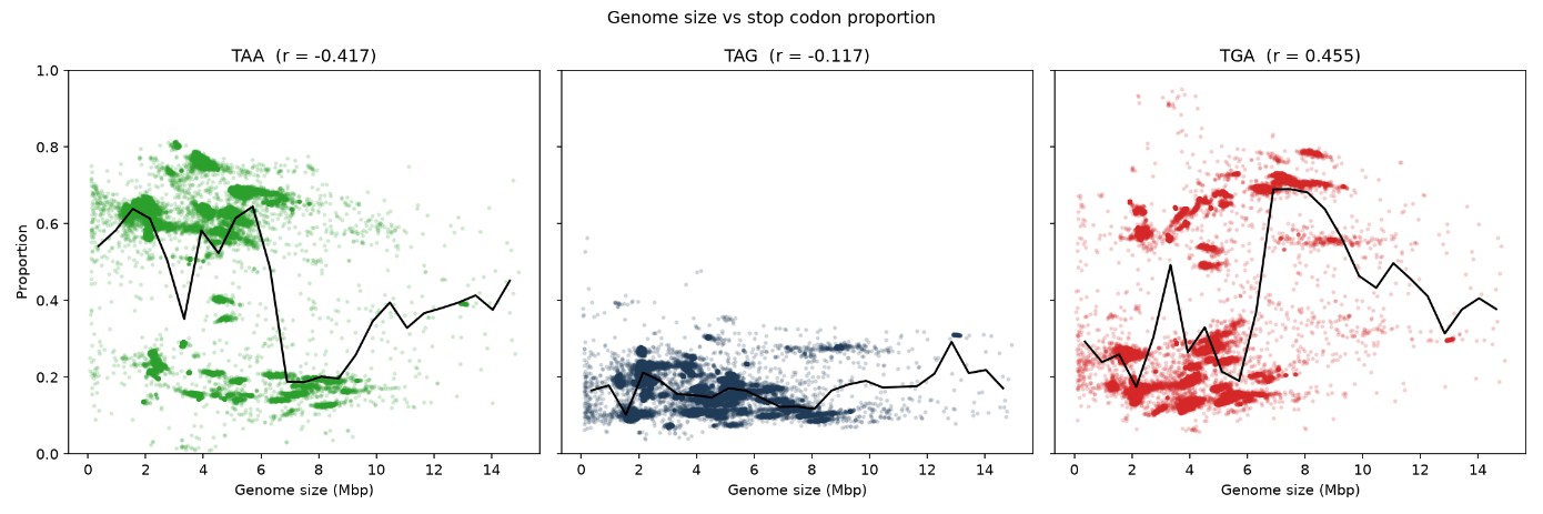
Genome size looks like it matters: r = -0.417 for TAA and r = 0.455 for TGA, with TAA holding near 0.58-0.62 up to 5 Mbp, dropping sharply between 6 and 8 Mbp as TGA climbs to 0.64-0.66, then partially recovering above 9 Mbp.

It does not survive a control. GC content and genome size are themselves correlated at r = 0.708 in this dataset, because the largest genomes here belong to GC-rich species such as Burkholderia. Holding GC constant with a species-level partial correlation collapses the genome size to TAA association to r = 0.048. Once base composition is accounted for, genome size carries almost no signal of its own.

The extremes are also not believable genomes. 228 assemblies fall below 1 Mbp, the smallest a 67.5 kb fragment carrying 100 CDS, and the largest is a 14.93 Mbp assembly split across 9,115 contigs, far more likely contaminated than genuinely large.

The most interesting finding is not about biology. The headline frequencies depend on how the dataset is weighted: TAA is the most common stop codon when every genome counts equally, but TGA is the most common when every species counts equally.

The sample is why. Streptococcus pneumoniae alone accounts for 70,851 of the 202,388 genomes; the three most represented species account for 58.8% and the ten most for 88.7%. The genome counts are dominated by AT-rich pathogens, while the species roster leans GC-rich because 86 of the 207 named labels are represented by a single genome. Neither weighting is unbiased, and the true domain-wide values must sit somewhere between them.

There is a corroborating detail. Korkmaz et al. report TAG at roughly 20% across the GC range. The species-weighted figure here is 0.198, which matches closely; the genome-weighted figure of 0.168 does not. A large dataset is not automatically a representative one.

One genus refuses to follow the pattern. Bradyrhizobium japonicum averages a TAG proportion of 0.280 and B. diazoefficiens 0.278, with related species also well above the dataset average, all at GC contents of 63-64% where TGA would normally dominate. Base composition does not explain it, which points instead at the release factor complement in the lineage. It is the clearest candidate in the dataset for a follow-up.

No invalid triplet was recorded anywhere in 536 million coding sequences. That figure needs reading carefully rather than celebrating. Bakta annotates coding sequences as open reading frames that end in a stop codon, so a valid triplet is what you would expect by construction, and a zero count is not on its own evidence that the extraction is biologically correct.

What it does rule out is a systematic fault. An off-by-one error converting Bakta's one-based inclusive coordinates, a mishandled negative strand, or a failed contig lookup would each have produced a large invalid rate, and at this scale none of them is present.

Treating each genome as an independent data point is the main statistical weakness. Genomes from one species share an evolutionary history, so analysing 202,388 of them without accounting for phylogenetic structure inflates the effective sample size and likely exaggerates the correlations. Species-level averages, or a phylogenetically adjusted method such as PGLS, would be more defensible.

Coverage has real holes. Only 1,124 genomes, 0.56% of the total, and four of the 207 named species fall between 49% and 57% GC, which is exactly where the TAA/TGA crossover sits. Escherichia, Salmonella, Pseudomonas aeruginosa, Staphylococcus aureus and Mycobacterium are absent from the dataset entirely, and those are the mid-GC organisms that would fill the gap.

Assembly quality was filtered only indirectly, since Bakta's PASS status certifies the annotation rather than the assembly. Applying a modest screen afterwards, at least 1 Mbp, no more than 500 contigs, named species only, removes 2.8% of the data and barely moves the results: TAA goes from 56.45% to 56.91% and the GC/TAA correlation from -0.855 to -0.849. The conclusions hold, but the screen should have been applied from the start.

One weakness was in the planning rather than the code. The codon counting was first implemented against GFF3 on the assumption that this was the format AllTheBacteria distributed. The annotations are Bakta JSON, and the parsing had to be rewritten. Opening a single annotation file before committing to a format would have avoided the whole cost.

Extending coverage into the 49-57% GC range is the most useful next step, since it closes the gap and brings in reference organisms like E. coli. Beyond that: species-level summaries as the unit of analysis, formal outlier detection using per-genome Z-scores against the genus mean, and an automated pytest suite built on the existing synthetic test file. The pipeline is already capable of all of it; what it needs is a broader and better chosen sample.